2004:03:15 FocLog.spt.

FocLog.spt is used to either extract and display head realtime head log data, or to read and display previously extracted head logs data.

If extracting data from the head, then it is assumed that the head log has already been acquired and the data is sitting in the head memory. Typically, this script is used for the case where the data is drum position synchronous. The script ReadLogData.spt is usually used for non drum position synchronous data.

The script is an interactive one, where you can plot graphs again and again until you are done. This script is supplied by the Th2 group.

When to run this script: Whenever you want to extract and display head log data in the form that this script provides, which is simple sample verses, sample index around drum with each swath overlaid, and/or sample verses swath at one drum index. The plot also does contour plots.

This script uses features only available in SPLOT version 3.95 and later. The script checks that your SPLOT version is new enough (even if it is within Service Shell), and will abort if not.

Instructions:

Note:if you want to log head data, you must already have the head log data captured before you run this script.

Use LogSetup.spt to setup the log for capture.
Plot or do plot headtest or whatever is needed to capture the log data.
Run this script and interact with the dialog boxes.
Note that it can take a long time over a dial-up connection to extract the entire log. Try to only ask for the amount of log needed for your application.
For your test try to note roughly where around the drum your sample starts and ends and where the clamps are. This will help you to identify media verses bare drum verses clamp areas on the graphs.

Simple Dialog boxes:

Getting Started	- This section explains how to get the data you wish to plot.
Choosing Plots	- This section explains how to choose what data you wish to plot.
Scaling	- This section explains how to scale your plot.
More views	- This section explains how to do a subscan plot and shift the x-axis of the plots.
New features	- This section explains new features available in FocLog.spt version 2.1 and it's derivative components.

Advanced Dialog boxes:

The Advanced Tab	- This section explains how to access the advanced options of the script.
Bidirectional Data	- This section explains how to deal with bidirectional data using the script.
Error Processing	- This section explains the various options to filter the Focus Error Data.
Predicted Swath	- This section explains how to show a predicted swath on the Lens Position Graph.
Contour Plots	- This section explains how to plot contours.
Advanced Outputs	- This section explains the advanced outputs available, writing time files and html files.

Simple Dialog Boxes

Getting Started

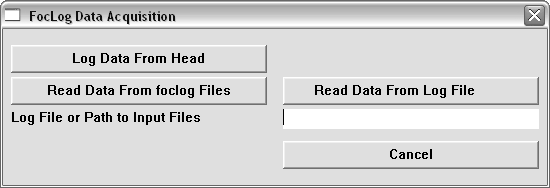
The first dialog box you see when you run the script is to decide where to get the data from, the head or from some previously saved data from a previous run of the script or a log file.

To load from previous foclog files, input the directory into the 'Log File or Path to Input Files' edit box and click the 'Read Data From foclog Files' button.
To load from a log file, input the path and filename into the 'Log File or Path to Input Files' edit box and click the 'Read Data From Log File' button.
The script informs the use of every thousandth line processed.

Notes for reading from a log file:	dErrorCal is set to 164.344 and dLPosCal is set to 10.009.
	Head Serial number is set to T99999
	The foclog files are stored in the directory containing the log

If you ask for data from the head, the second dialog asks for what percentage of the log starting from what percentage offset. The script will inform the user of every thousandth line acquired.

When you log data from the head it saves the foclog files automatically. The script then goes to the main dialog.
Back to top

Choosing Plots

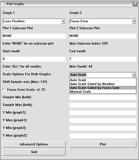
The next dialog box allows you to repeatedly plot two graphs at once (until you wish to quit) and determines the page contents, scaling, and displaying options. Every time a plot is made the plot is automatically saved as a graphical file whose type is defined by "#define TII_SAVEGRAPHTYPE" in localjig_include.spt . There is a pulldown menu for each graph, simply select the graph you want.

The dialog box also shows you the last swath value. You can choose to display any or all swaths in the range 0 to Max Swath.

Example 1: Capture during a plot - Quantum 800
The log was setup to trigger on imaging, with no delay, and record: Imaging, SUM, LPOS, Error, Focus gate.
The following graph is of swaths 4 to 7 of Lens Position and Focus Error.

The graph shows the swaths in up to 6 colours. If there are 6 or less swaths the legend displays them.
In the graph the two vertical blue lines that go as far outside the graphing area as the axis ticks are the focus gate signal overlaid on the graph.
In the graph the two vertical green lines that go as far outside the graphing area as the axis ticks are the newline and/or imaging signal overlaid on the graph.
The graphs always start at the active going edge of the newline and/or imaging signal. If you do not know what the signals NEWLINE and IMAGING are then this script is not intended for you.

Back to top

Scaling

There are 4 scaling options in this script. They can be chosen from the Scaling Options pickbox.

They are:

Auto Scale	- Default Scaling choice, scales the data based on the limits of the entire data set.
Auto Scale Gated By Newline	- This is the same as Auto Scale but only the data confined within the newline signal gate is used to scale the data.
Auto Scale Gated By Focus Gate	- This is the same as Auto Scale but only the data confined within the Focus signal gate is used to scale the data.
Manual	- Manual scaling allows you to put in specific values yourself into the fields below the scale choice menu. Note: If you don't enter some fields they will be automatically determined from the limits of the data (y = 0 reference will be an extrema unless otherwise specified).

Note: When the plot is a subscan plot and the scaling option is a gated autoscale, the scale will be determined by auto scaling (as gated makes no sense in this case). See More Views section for more.

The scale for the index around the drum depends on the type of sampling you did. Typically, take the DRUM R.P.M. and the maximum index around the drum to calculate the time of the X-Axis.
In this example the maximum index is 480, the drum rpm was 375 and there was a sample in the log that was at 3 KHz. So as a sanity check we will calculate the expected samples per revolution: That is 160 milliseconds per drum revolution or 480 samples at 3 KHz, so the numbers make sense.
It is best to look at a graph of the SUM signal to see if the timing makes sense (which I didn't provide here).
In these graphs, the focus beam is off plate for about 2/3 of the first swath (light blue). The plate curl is quite pronounced on this plate, which is why you see such a large lens position change over the first few swaths. The large focus tracking errors in the first few swaths result from the real time error calculation combining with the steep sub-scan slope and calculating error while it doesn't count for the extrapolated backwards swaths and the interpolated swath. By the time focus has transitioned to focus on, the error tracking error is reduced.
Outside of the focus gate area, we are not concerned with the focus error. The signal might be from drum for clamp in the imaging or newline inactive area. This is where the gated scale options are useful.

Another important scaling option is to lock the error scale to +/- 25 microns which is a very common and useful scale. This can be activated via the 'Focus Error Scale: +/- 25' checkbox. This will override any other scaling.

A plot is shown below using Autoscale gated by Focus Gate.

More Views

Subscan Plots
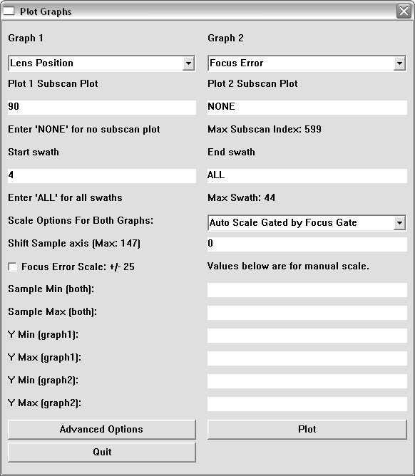
From the graph, it was desired to look at index 90 with time (for the lens position). I.E. we want to see the shape of the bump at index 90 verses swath number.
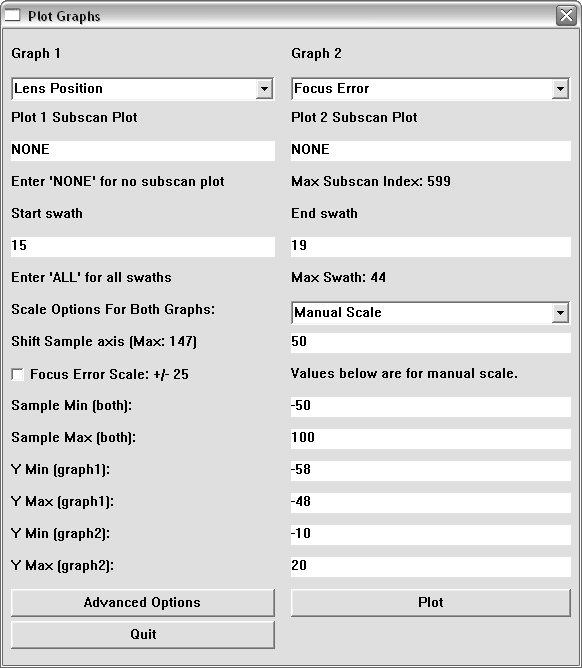
The dialog box for the graph was:

The dialog show you the maximum corner turn index.

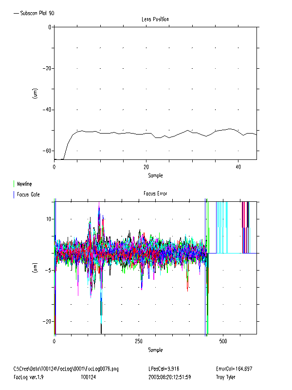
The resulting graph was:

The scaling option for the subscan graph is auto if a gated auto is selected because there is no gate on an index vs. time graph. The legend displays the index number.

Shifting the X axis
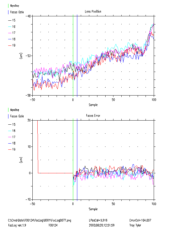
It may be desirable to shift the data so that the plot shows the lead in to the first newline at 0, this is done by entering a 'Shift X axis' value.
The dialog box for the graph was:

The dialog informs you of the maximum shift value (such that the trailing newline does not get wrapped). This graph was also done using manual scaling to show how it works.

The resulting graph was:

New Features for FocLog.spt version 2.1

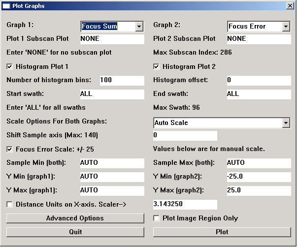
The simple and advanced dialog boxes have been reduced in vertical size from what is mainly shown in this help file, as they were too tall for easy use with some smaller screen configurations. An example of the new basic dialog box is shown below.
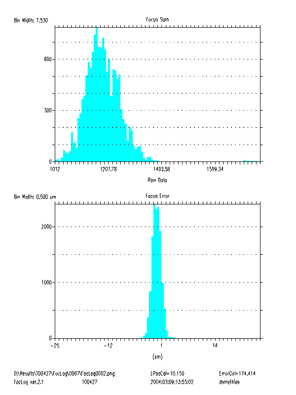
The simple dialog box for FocLog.spt version 2.1 has a few new buttons and inputs added. Histograms of the log data can now be made for the active image area. Histograms can be useful for comparing tracking error, SUM spread and such. An example histogram graph is included below as is an example of the Foclog 2.1 simple dialog box. The number of histogram bins is selectable, mainly to prevent bin aliasing (make the number of bins smaller if the histogram oscillates). Sometimes it is desirable to not inlcude leading and trailing edge problems in the histograms. The histogram offset is the number of samples to ignore at the leading and trailing edge for the histogram, in addition to the focus gate.
If possible, there is now an option to scale the x-axis in mm, rather than units of log samples. If you are reprocessing old data, then the x-axis scale will be 0, but you can edit the box if you know the appropriate value. If you are extracting a head log that was acquired earlier than the last plot that was run, then the script derived X-scale factor might be incorrect.
Sometimes the head data log does not fill up during a plot and or others problems occur that make the x-axis unreasonably large. Also some users do not want to see the lead-in and trail-out information. There is now a check box to force displaying of only the active image area ("Plot Image Region only"). This helps find, and zoom in on, the desired area to be graphed.
The entire bulk of FocLog.spt has been moved to the include file tii_FocLog.spt and the DLL file. Thus it is now easy to make a higher level script that just calls FocLog as a subroutine. Click here for a simple example script (as a text file) showing how to call FocLog as a subroutine.

The simple FocLog version 2.1 dialog box and the one used for the histogram graph:

The resulting example histogram graph was:

Advanced Dialog Boxes

The Advanced Tab

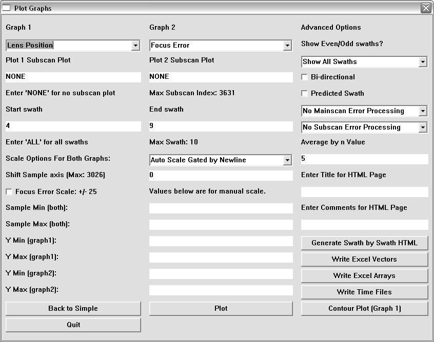
Clicking the "Advanced Options" button in the simple dialog box will open the advanced dialog box. This dialog box is shown in the picture below:

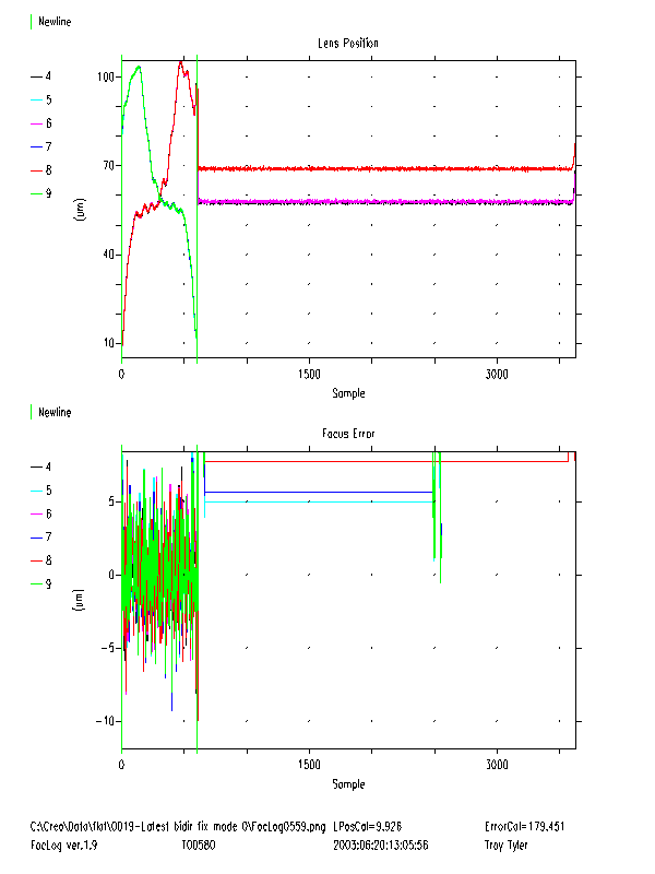
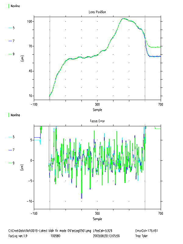
Example 2: Flat Bed plotter Data
The log was setup to trigger on imaging, with no delay, and record: Imaging, LPOS, Error, Focus Command LPOS.
The following graph is of swaths 4 to 9 of Lens Position and Focus Error.

Bidirectional Data

Bidirectional Checkbox
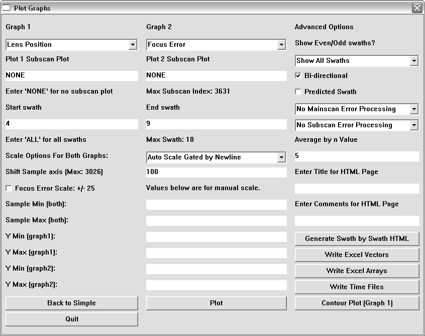
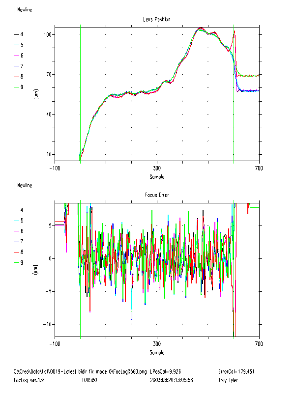
The data from Example 2 is bidirectional, so it is useful to have every odd swath flipped. Also the lead in and lead out from newline is controlled by the Shift X axis field. The dialog box for this plot is shown below:

The following graph was produced:

Show Even/Odd Swaths?
Since the servos for each direction are independent, it is useful to display the odd or even plots, as well as all the plots. Show odd/even also works for non bidirectional data. The odd swaths of the graph above are shown below.

Error Processing

It is desirable to filter the error signal, currently there is only one mainscan filter available, and no subscan filters. The mainscan filter option currently is a moving average filter by n samples. To use the filter select the filter